Typical applications

High-angle instability

A special treatment takes care of so-called high-angle instability (Ashton et al., 2001), which allows spits to develop. In cases where the local angle exceeds the critical angle on one side and is less than the critical angle at the updrift side, the transport at the downdrift point is set to the maximum transport (or the angle is set to the critical angle). fig-image003 illustrates the effect of this treatment, where a central scheme would lead to unstable behavior, the local upwind treatment ensures a smooth development into a spit. The physics in the model is the same as in Ashton et al. (2001, 2016), and Ashton and Murray (2006), and therefore it inherits most of the behavior of their Coastal Evolution Model. The novelty in ShorelineS is that it achieves the same behavior with a vector-based rather than a grid-based approach. This is more elegant and more efficient, especially when large areas need to be covered.

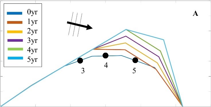
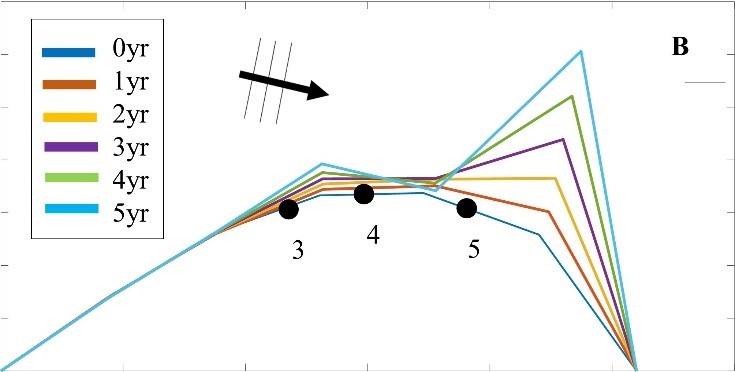
Example of high-angle instability with standard central scheme (A) and upwind scheme (B).

Barrier or spit overwash

For simulating barriers that already exist or that are in the form of developed spits due to high wave angle instability, it was necessary to represent the overwash process as it maintains the width of the barrier to a certain limit (Leatherman, 1979).

(Ashton & Murray, 2006) introduced the physical process of overwash by assuming a minimum barrier width such that sediment eroded from the seaward side is deposited on the landward side. By simultaneously retreating the seaward and landward sides of a section narrower than the specified critical width, the retreating section creates a longshore transport gradient that tends to fill it up; thus, the retreating helps maintain the width.

A similar concept was implemented in ShorelineS in a simple approach for treating the barrier width. At each time step, the model checks the local barrier width at each point/node, measured in the incident wave direction. If the barrier is narrower than the critical width, then overwash occurs. The overwash process moves the landward point a distance equal to the difference between the actual width and the critical width. Such a distance is not allowed to exceed a given percentage (e.g. 10%) of the local spatial discretization distance of the grid per time step to avoid discretization artefacts. Then the model looks for the closest node on the seaward side to erode it by the same amount (Figure SI02). A possible refinement is, as in Ashton and Murray (2006), to assume different profile depths on the seaward and landward sides, as is logical in some settings, e.g., for the case of an eroding barrier island. In this case the landward extension would be larger than the erosion on the seaward side.

Merging and splitting

One of the advantages of the ShorelineS model is that it can simulate multiple coastal sections at the same time, and these sections can affect each other by shielding the waves. Small parts of the coast are allowed to split and migrate as the spits are growing and in some cases break up and migrate as a small island. An example of the splitting procedure is shown in Figure SI03. Such splitting typically happens when the seaward side of a section erodes by more than the overwashing process allows for or when the latter is not activated. The numbering is indicated to show how the grid cell connections change after the splitting procedure: from one continuous coastline section to two separately numbered sections.

If two sections intersect, they may merge into one section as the simulation continues, as is illustrated in Figure SI04. Such merging typically happens due to shoreward migration or extension of a spit towards the mainland coast. Again, the numbering is included to indicate how the separate spit and mainland coast sections are now joined at the seaward side as a continuous coastline numbered 12-20 and a lagoon numbered 1-10.

Treatment of groynes

Groynes can be treated simply as any structure crossing the coastline, where the transport at the transport point closest to the intersection between the structure polyline and the coastline is set to zero. However, such a treatment does not give a very accurate representation of the groyne position and local coastline evolution, and does not account for bypassing in a smooth way. Therefore, a more eleborate treatment was presented in Ghonim (2019), which is summarized as follows. First, additional grid points exactly on either side of each groyne are introduced. Second, the local coastline position at either side of the groyne is forced to move along the groyne. Third, bypassing and transmission are accounted for, according to the following mechanisms.

Bypassing can be simulated in two ways, either as starting only when the updrift accretion has reached the tip of the groyne, or gradually increasing if the depth at the tip of the groyne is less than the depth of active transport. The first approach follows the considerations of , assuming a fully impermeable structure, such as a groyne with complete blockage of the longshore transport. Sand bypassing takes place only when the groyne is filled with sand. Based on that, the longshore sediment transport is set to zero at the structure and the sand bypassing factor (BPF) also is set to zero from the start of the simulation until the moment when the sediment reaches the tip of the groyne. Then, the bypassing factor is set to its maximum value (BPF=1), which means that all sediment bypasses the groyne’s tip and moves towards its downdrift side. In that case the lateral boundary condition at grid point i (see Figure SI05), which is located at the groyne representing the bypassed volume can be expressed as:

where QSi is the longshore transport at grid point i. There were many options for how the bypassed sediment should be distributed downdrift of the groyne. The most appropriate distribution of the bypassed sediment, in line with the expected flow pattern around the groyne, which attaches roughly at the end of the sheltered area, is to pass all the bypassed sediment at the last sheltered grid point ilast and to leave the sheltered area untouched. To do so numerically, the lateral boundary conditions at the downdrift side of the groyne are set as follows:

Eq. (11) ensures that only the last sheltered grid point obtains all the bypassed sediment and equal signs indicate that there is no sediment transport gradient from the grid point i to the last sheltered grid point ilast. This approach keeps the sheltered grid points fixed in their positions except for the last one, which gives a transport gradient to its following grid point.

That this treatment is more realistic than the classical Pelnard-Considère solution where an erosion peak at the downdrift end of the groyne is assumed follows from many examples worldwide, where the erosion peak is rarely found right next to the groyne but always some distance downdrift, due to the wave sheltering and recirculation in this area. An example is shown in Figure SI06, for a groyne field at Eastbourne, UK.

The second approach (Larson et al., 1987) assumes that sand bypassing does not take place only when the groyne is totally filled with sand, but it may take place just after the construction of the groyne. While sand moves along the coastline, it is influenced by the presence of the shore-normal structures, such as groynes and the response of the coastline to those structures varies for different locations and different types of structures. The main parameters that influence the response of the shoreline at the structure are the structure permeability and the bypassing ratio, which is the ratio between the water depth at the head of the structure Ds and the water depth of the active longshore transport DLT. The bypassing ratio varies between 0 and 1 (Hanson & Kraus, 2011).

Sand bypassing occurs at the seaward end of the groyne as long as Ds is less than DLT. The depth of the active longshore transport is similar to the depth of the highest 1/10 waves at the updrift side of the structure (Hanson, 1989), and represents the time-dependent depth for longshore sediment transport, which is often less than closure depth Dc, and can be estimated as:

where Aw = 1.27, a factor that converts the 1/10 highest wave height to significant wave height [-]; γ is the breaker index, the ratio between wave height to wave depth at breaking line [-] and (H1/3)b is the significant wave height at the line of breaking [m].

Based on the assumption of equilibrium profile shape (Dean, 1991), the water depth at the structure’s head Ds can be determined as:

where Ap is the sediment scale parameter [m^1/3] and ystr is the distance from the structure’s head to the nearest point of the coastline [m]. In that case, the bypassing factor (BPF) is estimated based on the following equation:

and the bypassing volume increases until reaching its maximum value when the groyne is filled with sediment [BPF =1]. The lateral boundary conditions at the groyne are otherwise equal to those for the first approach, as given by Eqs. (6) and (7).