How the model works
Introduction
To overcome the severe limitations of existing coastline models with a
fixed reference line, while avoiding the complexities of grid-based
approaches and geometrically complex volume reconstructions, a new
Shoreline Simulation model (ShorelineS) was developed, which is aimed at
predicting coastline evolution over periods of years to centuries. Its
description of coastlines is of strings of grid points (see fig-image001)
that can move around, expand and shrink freely. The coastline points are
assumed to be representative of the movement of the active coastal
profile, and hence are situated at the MSL contour. The model can have
multiple sections which may be closed (islands, lagoons). Sections can
develop spits and other features and they may break up or merge as the
simulation continues.
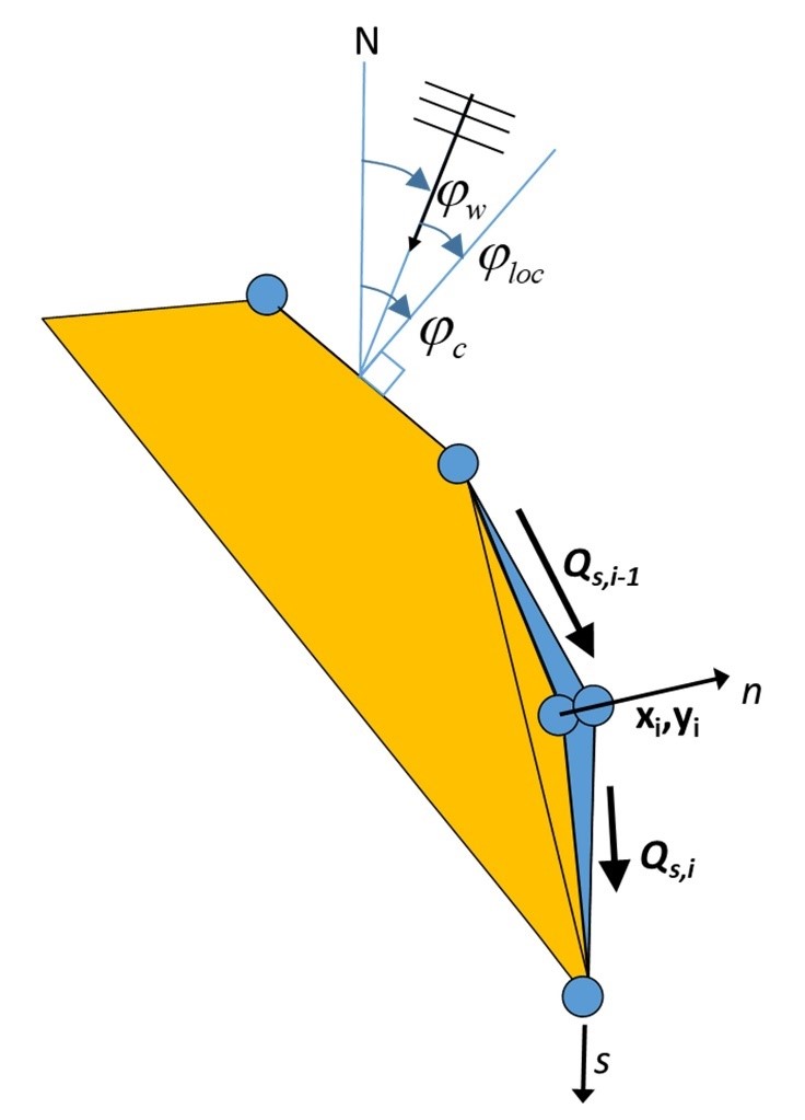
Coastline-following coordinate system and definition of wave and coast angles. \(\varphi_{c}\) is the orientation of the shore normal with respect to North; \(\varphi_{w}\) is the angle of incidence of the waves with respect to North and \(\varphi_{loc}\) is the local angle between waves and coast, defined as \(\varphi_{c} - \varphi_{w}\).
Basic equation
The basic equation for the updating of the coastline position is based on the conservation of sediment:
where n is the cross-shore coordinate, s the longshore coordinate, t is time, Dc is the active profile height, Qs is the longshore transport (m3/yr), tan β is the average profile slope between the dune or barrier crest and the depth of closure, RSLR is the relative sea-level rise (m/yr) and qi is the source/sink term (m3/m/yr) due to cross-shore transport, overwashing, nourishments, sand mining and exchanges with rivers and tidal inlets. In the Volume Balance section in the Supplementary Information we explain why equation correctly represents the balance of both dry land area and the sediment volume, even for curved coasts.
Transport formulations
The coastline changes are driven by wave-driven longshore transport,
which is computed using a choice of formulations, which can be
calibrated to match the local transport rates. The formulations listed
in Table 1 have been implemented. The definitions of the angles are as
in fig-image001.
CERC1 and CERC2 are defined in terms of the offshore wave angle, and CERC3 and KAMP are defined in terms of the breaking wave angle. However, in all cases the transport follows a shape rather similar to CERC1 when plotted against the deep water wave angle, with a maximum occurring at an offshore angle of 40° to 45° from wave incidence.
CERC1 is the simplest formula and is mainly meant for illustrating the principles of the behavior of the coastline model. CERC2 is derived from the official CERC formula to formally include the effect of refraction and shoaling. Though its behavior is quite similar to CERC1, it allows for a direct comparison with the Coastal Evolution model that utilises it. The CERC3 and KAMP formulas are widely used in models worldwide such as GENESIS or UNIBEST and again can be useful for intercomparison with such models. CERC1, CERC2 and CERC3 have a single calibration coefficient, whereas the KAMP formula requires, usually uncertain, extra inputs such as beach slope and grain size but has the ambition to be a more accurate, predictive formula.
In tab-Implemented-longshore-transport, HS0 and Hsb are the significant wave height at the
offshore location and point of breaking respectively (m), T is the
peak wave period (s), D50 is the median grain diameter (m), mb
is the mean bed slope (beach slope in the breaking zone), Φloc is
the relative angle of wave incidence for waves offshore and Φlocb is
the relative angle of waves at the breaking point; b and K2 are
the calibration coefficients of CERC1 and CERC2 formulations
respectively, which are computed as :.
where k is the default calibration coefficient according to the Shore Protection Manual (USACE, 1984), ρ the density of the water (kg/m3), ρs the density of the sediment (kg/m3), g the acceleration of gravity (m/s2) and γ the breaker criterion.
Numerical implementation
The ShorelineS model is implemented in Matlab. The flow diagram of the
model is depicted in fig-image002. In the following we will describe the
procedure point by point.

Flow diagram of the ShorelineS model.
The coastline positions are given in two column vectors xmc and ymc, where the different coast sections are separated by NaN’s. The sea is defined to the left when following the coastline positions. If a section ends at the same coordinates as where it starts, it is treated as a cyclic section and may represent either an island or a closed lagoon. The coordinates may be in any Cartesian (metric) system. Structures are defined in a similar way, as two column vectors where different structures may be defined, separated by NaN’s.
The offshore wave climate can be specified in three ways:
By means of wave direction and a spreading sector, where a uniform distribution is assumed between the mean wave direction and plus or minus half the spreading sector. For each time step a random wave direction will be chosen from this sector.
By a wave climate consisting of a number of wave conditions characterized by significant wave height, peak period and mean wave direction, each with equal probability of occurrence. A condition will be chosen randomly for each time step.
By a time series of these wave conditions, from which the model will interpolate in time.
Various lateral boundary conditions were implemented in the model to represent a variety of coastal situations. For the non-cyclic sections the lateral boundary conditions are specified by controlling the sediment transport rate at the start and end of the boundary, thereby specifying a constant coastline position, a constant coastline orientation or a periodic boundary condition. One type of boundary condition is applied at all open-ended sections, whether existing or newly created. The model detects when a section end point is near the section start point and then always applies cyclic boundary conditions.
Nourishments can be prescribed through a number of polygons within which each nourishment takes place, start and end times, and the total volume of each nourishment. This information is then internally converted into a shoreline accretion rate by dividing the total volume by the time period, the length of coastline within the polygon and the profile height, Dc. By the same mechanism sediment discharged by a river can be distributed over a coastline section within a specified polygon. Shoreline recession as a result of relative sea level rise can be specified, e.g., resulting from the Bruun rule (Bruun, 1962), as given by eq. .
All inputs are collected in a single structure S that is passed on to the main function ShorelineS. Preparation of the input can be done in a tailor-made script, but ShorelineS and its sub-functions normally do not have to be altered for a specific application. The main function ShorelineS contains default values for all inputs that are not application-dependent.
The cumulative distance s along each coast section is computed, and this is then distributed over equidistant longshore grid cells based on a given initial grid size. The x and y positions of the coastline then are interpolated along s to obtain the x and y positions of the grid points.
In cases where the grid sizes expand (e.g., at the tip of an expanding spit), new grid points are inserted where the grid size exceeds twice the initial prescribed grid size. Where the grid distances shrink (e.g., at an infilling bay or a shrinking spit) grid points are removed when the grid distance becomes less than half the original grid size.
To avoid strong variations in grid size after inserting or extracting grid cells in expanding or shrinking sections, some smoothing of the s-grid is applied. The smoothing factor has to be chosen carefully as too much smoothing may lead to a loss of planform area and will tend to straighten out sections that should not move at all. The smoothing formulation applied is a simple 3-point smoothing according to:
where f is a smoothing factor, with default value of 0.1. Smoothing can lead to losses in the sediment balance and in situations where this is critical a value closer to zero is advised.
The local wave angle is estimated through the wave transformation from deep water to the nearshore using Snell’s law of refraction and from the nearshore to the breaking line using the equations of van Rijn (2014). The refraction from deep water to the toe of the dynamic profile can be done based on the assumption of parallel offshore depth contours, or using a 2D refraction model to provide alongshore-varying wave conditions.
Some parts of the coastline might be sheltered by structures or other parts (sections) of the coast. Hard structures or rocky shores are represented by an arbitrary number of polylines, which shield waves and block longshore transport where they cross a coastline. Thus, sea walls, hard rocks and headlands can represent supply-limited situations where the transport is determined by the updrift sand supply and ‘plugs’ of sand are bypassed. The waves at any location can be shielded by other coast sections or hard structures, see Figure SI01. This approach is valid when the scale of the structures is much larger than the wave length; if this is not the case, diffraction can be activated using different approximations (Elghandour, 2018).
Given the local wave angle with respect to the coast normal and the refracted wave conditions (or deep water wave directions in the case of the CERC1 and CERC2 formulas) the longshore transport can be computed atdelta each transport point between two adjacent coastline points. At present, a choice of formulations as listed in Table 1 is available to be used.
Coastline evolution
At each point the local direction of the coast is determined from the
two adjacent points (as a reference line), then the longshore transport
is calculated for each segment. The difference leads the points to build
out or to shrink. The mass conservation equation is solved using a
staggered forward time–central space explicit scheme (see fig-image001):
where j is the time step index, \(\delta t\)is the time step (yr), i is the point/node index and Li is the length of the considered grid element computed from \(L_{i} = \sqrt\{(x_{i + 1} - x_{i - 1})^{2} + (y_{i + 1} - y_{i - 1})^{2}}\)and xi and yi are the Cartesian coordinates of point i. From the normal displacement it follows that the change in position of point i then becomes:
The scheme can be shown to be conserving the land area. Since an explicit scheme is applied, the time step is limited by the following criterion (Vitousek & Barnard, 2015):
where the diffusivity :math: varepsilon is related to the maximum gradient of the sediment transport with respect to the wave angle relative to the coast, which can be approximated by:
where Qmax is the maximum transport rate in the model.
Therefore the following is obtained:
This criterion can be restrictive for small grid sizes (e.g. less than 100m). Stability is, however, guaranteed through this adaptive timestep.